Basic SHAP Interaction Value Example in XGBoost
This notebook shows how the SHAP interaction values for a very simple function are computed. We start with a simple linear function, and then add an interaction term to see how it changes the SHAP values and the SHAP interaction values.
[1]:
import numpy as np
import xgboost
from sklearn.linear_model import LinearRegression

import shap
Explain a linear function with no interactions
Simulate some binary data and a linear outcome with an interaction term.
Note we make the features in X perfectly independent of each other to make it easy to solve for the exact SHAP values.
[2]:
N = 2_000
X = np.zeros((N, 5))

X[:1_000, 0] = 1

X[:500, 1] = 1
X[1_000:1_500, 1] = 1

X[:250, 2] = 1
X[500:750, 2] = 1
X[1_000:1_250, 2] = 1
X[1_500:1_750, 2] = 1

# mean-center the data
X[:, 0:3] -= 0.5

y = 2 * X[:, 0] - 3 * X[:, 1]
We see that the variables are indeed independent
[3]:
np.cov(X.T)
[3]:
array([[0.25012506, 0.        , 0.        , 0.        , 0.        ],
       [0.        , 0.25012506, 0.        , 0.        , 0.        ],
       [0.        , 0.        , 0.25012506, 0.        , 0.        ],
       [0.        , 0.        , 0.        , 0.        , 0.        ],
       [0.        , 0.        , 0.        , 0.        , 0.        ]])
and mean-centered.
[4]:
X.mean(axis=0)
[4]:
array([0., 0., 0., 0., 0.])
[5]:
# train a model with single tree
Xd = xgboost.DMatrix(X, label=y)
model = xgboost.train({"eta": 1, "max_depth": 3, "base_score": 0, "lambda": 0}, Xd, 1)

print("Model error =", np.linalg.norm(y - model.predict(Xd)))
print(model.get_dump(with_stats=True)[0])
Model error = 0.0
0:[f1<0] yes=1,no=2,missing=1,gain=4500,cover=2000
        1:[f0<0] yes=3,no=4,missing=3,gain=1000,cover=1000
                3:leaf=0.5,cover=500
                4:leaf=2.5,cover=500
        2:[f0<0] yes=5,no=6,missing=5,gain=1000,cover=1000
                5:leaf=-2.5,cover=500
                6:leaf=-0.5,cover=500
SHAP values
[6]:
pred = model.predict(Xd, output_margin=True)

explainer = shap.TreeExplainer(model)
explanation = explainer(Xd)

shap_values = explanation.values
# make sure the SHAP values add up to marginal predictions
np.abs(shap_values.sum(axis=1) + explanation.base_values - pred).max()
[6]:
0.0
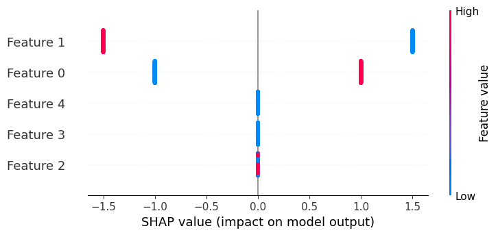
If we build a beeswarm plot, we see that only features 0 and 1 have any effect on the output, and that their effects only have two possible magnitudes (1/-1 and 1.5/-1.5 correspondingly).
[7]:
shap.plots.beeswarm(explanation)
Train a linear model
[8]:
lr = LinearRegression()
lr.fit(X, y)
lr_pred = lr.predict(X)
lr.coef_.round(2)
[8]:
array([ 2., -3., -0., 0., 0.])
Make sure the computed SHAP values match the true SHAP values (we can compute the true SHAP values directly for any linear regression)
[9]:
main_effect_shap_values = lr.coef_ * (X - X.mean(0))
np.linalg.norm(shap_values - main_effect_shap_values)
[9]:
1.6542433490447965e-13
SHAP interaction values
Note that when there are no interactions present, the SHAP interaction values are just a diagonal matrix with the SHAP values on the diagonal.
[10]:
shap_interaction_values = explainer.shap_interaction_values(Xd)
shap_interaction_values[0]
[10]:
array([[ 1. ,  0. ,  0. ,  0. ,  0. ],
       [ 0. , -1.5,  0. ,  0. ,  0. ],
       [ 0. ,  0. ,  0. ,  0. ,  0. ],
       [ 0. ,  0. ,  0. ,  0. ,  0. ],
       [ 0. ,  0. ,  0. ,  0. ,  0. ]], dtype=float32)
Let’s ensure that the SHAP interaction values sum to the marginal predictions:
[11]:
np.abs(shap_interaction_values.sum((1, 2)) + explainer.expected_value - pred).max()
[11]:
0.0
And ensure the main effects from the SHAP interaction values match those from a linear model:
[12]:
total = 0
for i in range(N):
    for j in range(5):
        total += np.abs(shap_interaction_values[i, j, j] - main_effect_shap_values[i, j])
total
[12]:
1.0533118387982904e-11
Explain a linear model with one interaction
Simulate some binary data and a linear outcome with an interaction term.
Note that we make the features in X perfectly independent of each other to make it easy to solve for the exact SHAP values.
[13]:
N = 2_000
X = np.zeros((N, 5))
X[:1_000, 0] = 1

X[:500, 1] = 1
X[1_000:1_500, 1] = 1

X[:250, 2] = 1
X[500:750, 2] = 1
X[1_000:1_250, 2] = 1
X[1_500:1_750, 2] = 1

X[:125, 3] = 1
X[250:375, 3] = 1
X[500:625, 3] = 1
X[750:875, 3] = 1
X[1_000:1_125, 3] = 1
X[1_250:1_375, 3] = 1
X[1_500:1_625, 3] = 1
X[1_750:1_875, 3] = 1

# we can't exactly mean center the data or XGBoost has trouble finding the splits
X[:, :4] -= 0.4999

# interaction of features is implemented as the multiplication of the features. Note that any other function of the
#  features would also work, but is harder to interpret (e.g. sin(x1*x2)).
y = 2 * X[:, 0] - 3 * X[:, 1] + 2 * X[:, 1] * X[:, 2]
[14]:
X.mean(axis=0)
[14]:
array([1.e-04, 1.e-04, 1.e-04, 1.e-04, 0.e+00])
[15]:
# train a model with single tree
Xd = xgboost.DMatrix(X, label=y)
model = xgboost.train({"eta": 1, "max_depth": 4, "base_score": 0, "lambda": 0}, Xd, 1)
print("Model error =", np.linalg.norm(y - model.predict(Xd)))
print(model.get_dump(with_stats=True)[0])
Model error = 1.7365037830677591e-06
0:[f1<0.000100001693] yes=1,no=2,missing=1,gain=4499.3999,cover=2000
        1:[f0<0.000100001693] yes=3,no=4,missing=3,gain=1000.00024,cover=1000
                3:[f2<0.000100001693] yes=7,no=8,missing=7,gain=124.950005,cover=500
                        7:leaf=0.99970001,cover=250
                        8:leaf=-9.99800031e-05,cover=250
                4:[f2<0.000100001693] yes=9,no=10,missing=9,gain=124.950195,cover=500
                        9:leaf=2.99970007,cover=250
                        10:leaf=1.99989998,cover=250
        2:[f0<0.000100001693] yes=5,no=6,missing=5,gain=999.999756,cover=1000
                5:[f2<0.000100001693] yes=11,no=12,missing=11,gain=125.050049,cover=500
                        11:leaf=-3.0000999,cover=250
                        12:leaf=-1.99989998,cover=250
                6:[f2<0.000100001693] yes=13,no=14,missing=13,gain=125.050018,cover=500
                        13:leaf=-1.00010002,cover=250
                        14:leaf=0.000100019999,cover=250
SHAP values
[16]:
pred = model.predict(Xd, output_margin=True)

explainer = shap.TreeExplainer(model)
explanation = explainer(Xd)

shap_values = explanation.values
# make sure the SHAP values add up to marginal predictions
np.abs(shap_values.sum(axis=1) + explanation.base_values - pred).max()
[16]:
4.7683716e-07
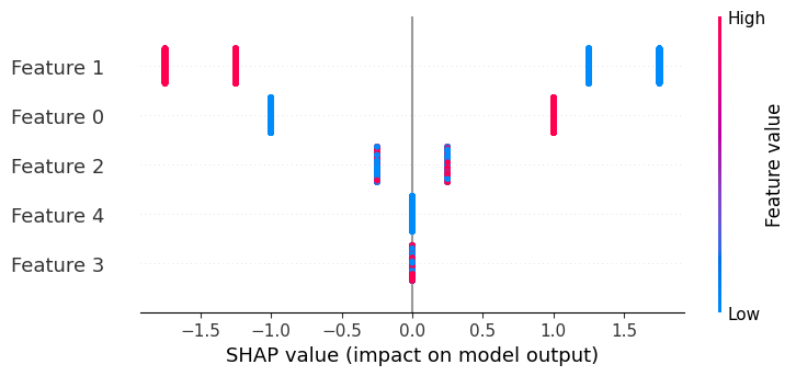
If we build a beeswarm plot, we see that now only features 3 and 4 don’t matter, and that feature 1 can have four possible effect sizes due to interactions.
[17]:
shap.plots.beeswarm(explanation)
Train a linear model
[18]:
lr = LinearRegression()
lr.fit(X, y)
lr_pred = lr.predict(X)
lr.coef_.round(2)
[18]:
array([ 2., -3., 0., -0., 0.])
Note that the SHAP values no longer match the main effects because they now include interaction effects.
[19]:
main_effect_shap_values = lr.coef_ * (X - X.mean(0))
np.linalg.norm(shap_values - main_effect_shap_values)
[19]:
15.811387829626835
SHAP interaction values
SHAP interaction contributions are displayed on the off-diagonal
[20]:
shap_interaction_values = explainer.shap_interaction_values(Xd)
shap_interaction_values[0].round(2)
[20]:
array([[ 1.  ,  0.  ,  0.  ,  0.  ,  0.  ],
       [ 0.  , -1.5 ,  0.25,  0.  ,  0.  ],
       [ 0.  ,  0.25,  0.  ,  0.  ,  0.  ],
       [ 0.  ,  0.  ,  0.  ,  0.  ,  0.  ],
       [ 0.  ,  0.  ,  0.  ,  0.  ,  0.  ]], dtype=float32)
Ensure the SHAP interaction values sum to the marginal predictions
[21]:
np.abs(shap_interaction_values.sum((1, 2)) + explainer.expected_value - pred).max()
[21]:
4.7683716e-07
While the main effects no longer match the SHAP values when interactions are present, they do match the main effects (from the linear model) on the diagonal of the SHAP interaction value matrix.
[22]:
total = 0
for i in range(N):
    for j in range(5):
        total += np.abs(shap_interaction_values[i, j, j] - main_effect_shap_values[i, j])
total
[22]:
0.0005347490392160024
[23]:
shap.dependence_plot(0, shap_values, X)
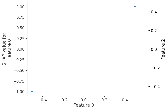
If we build a dependence plot for feature 0, we see that it only takes two values and that these values are entirely dependent on the value of the feature. Hence, they lie on a straight line (the value of feature 0 entirely determines its effect because it has no interactions with other features).
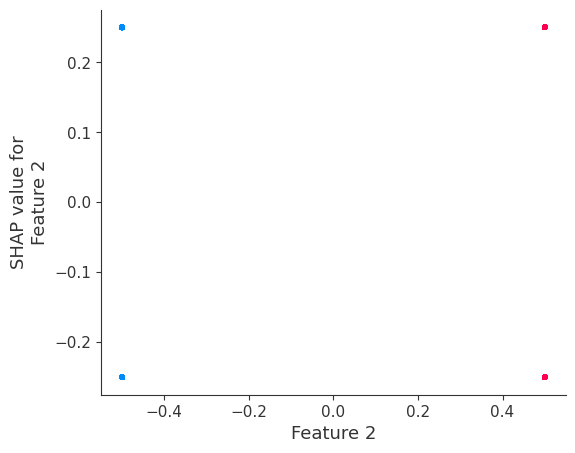
In contrast, if we build a dependence plot for feature 2, we see that it takes 4 possible values and they are not entirely determined by the value of feature 2. Instead they also depend on the value of feature 3. This vertical spread in a dependence plot represents the effects of non-linear interactions.
[24]:
shap.dependence_plot(2, shap_values, X)
invalid value encountered in divide
invalid value encountered in divide