SHAP Values for Multi-Output Regression Models
Author: coryroyce
Date updated: 3/4/2021
Create Multi-Output Regression Model
Create Data
Import required packages
[1]:
import pandas as pd
from keras.layers import Dense
from keras.models import Sequential
from sklearn.datasets import make_regression
Create a custom function that generates the multi-output regression data. Note: Creating 5 outputs/targets/labels for this example, but the method easily extends to any number or outputs.
[2]:
def get_dataset():
    # Create sample data with sklearn make_regression function
    X, y = make_regression(n_samples=1000, n_features=10, n_informative=7, n_targets=5, random_state=0)

    # Convert the data into Pandas Dataframes for easier maniplution and keeping stored column names
    # Create feature column names
    feature_cols = [
        "feature_01",
        "feature_02",
        "feature_03",
        "feature_04",
        "feature_05",
        "feature_06",
        "feature_07",
        "feature_08",
        "feature_09",
        "feature_10",
    ]

    df_features = pd.DataFrame(data=X, columns=feature_cols)

    # Create lable column names and dataframe
    label_cols = ["labels_01", "labels_02", "labels_03", "labels_04", "labels_05"]

    df_labels = pd.DataFrame(data=y, columns=label_cols)

    return df_features, df_labels
Create Model
Create a Tensorflow/Keras Sequential model.
[3]:
def get_model(n_inputs, n_outputs):
    model = Sequential()
    model.add(Dense(32, input_dim=n_inputs, kernel_initializer="he_uniform", activation="relu"))
    model.add(Dense(n_outputs, kernel_initializer="he_uniform"))
    model.compile(loss="mae", optimizer="adam")
    return model
Train Model
Create the dataset with the function defined above.
[4]:
# Create the datasets
X, y = get_dataset()

# Get the number of inputs and outputs from the dataset
n_inputs, n_outputs = X.shape[1], y.shape[1]
Load the model with function defined above.
[5]:
model = get_model(n_inputs, n_outputs)
Train the model
[6]:
model.fit(X, y, verbose=0, epochs=100)
[6]:
<tensorflow.python.keras.callbacks.History at 0x7f08e9a7e490>
Get model evaluation metrics to confirm training went well.
[7]:
model.evaluate(x=X, y=y)
32/32 [==============================] - 0s 826us/step - loss: 15.8952
[7]:
15.895209312438965
Model Prediction
Manual data can be entered but in this case, just us an arbitrary index form the feature/X data.
[8]:
model.predict(X.iloc[0:1, :])
[8]:
array([[ -15.026388,  -64.4412  ,  -75.39472 ,  -70.4628  , -126.55638 ]],
      dtype=float32)
Get SHAP Values and Plots
Apply Shapley vaules to the model.
[9]:
!pip install shap
import shap

# print the JS visualization code to the notebook
shap.initjs()
Collecting shap
  Downloading https://files.pythonhosted.org/packages/b9/f4/c5b95cddae15be80f8e58b25edceca105aa83c0b8c86a1edad24a6af80d3/shap-0.39.0.tar.gz (356kB)
     |████████████████████████████████| 358kB 6.0MB/s
Requirement already satisfied: numpy in /usr/local/lib/python3.7/dist-packages (from shap) (1.19.5)
Requirement already satisfied: scipy in /usr/local/lib/python3.7/dist-packages (from shap) (1.4.1)
Requirement already satisfied: scikit-learn in /usr/local/lib/python3.7/dist-packages (from shap) (0.22.2.post1)
Requirement already satisfied: pandas in /usr/local/lib/python3.7/dist-packages (from shap) (1.1.5)
Requirement already satisfied: tqdm>4.25.0 in /usr/local/lib/python3.7/dist-packages (from shap) (4.41.1)
Collecting slicer==0.0.7
  Downloading https://files.pythonhosted.org/packages/78/c2/b3f55dfdb8af9812fdb9baf70cacf3b9e82e505b2bd4324d588888b81202/slicer-0.0.7-py3-none-any.whl
Requirement already satisfied: numba in /usr/local/lib/python3.7/dist-packages (from shap) (0.51.2)
Requirement already satisfied: cloudpickle in /usr/local/lib/python3.7/dist-packages (from shap) (1.3.0)
Requirement already satisfied: joblib>=0.11 in /usr/local/lib/python3.7/dist-packages (from scikit-learn->shap) (1.0.1)
Requirement already satisfied: python-dateutil>=2.7.3 in /usr/local/lib/python3.7/dist-packages (from pandas->shap) (2.8.1)
Requirement already satisfied: pytz>=2017.2 in /usr/local/lib/python3.7/dist-packages (from pandas->shap) (2018.9)
Requirement already satisfied: setuptools in /usr/local/lib/python3.7/dist-packages (from numba->shap) (54.0.0)
Requirement already satisfied: llvmlite<0.35,>=0.34.0.dev0 in /usr/local/lib/python3.7/dist-packages (from numba->shap) (0.34.0)
Requirement already satisfied: six>=1.5 in /usr/local/lib/python3.7/dist-packages (from python-dateutil>=2.7.3->pandas->shap) (1.15.0)
Building wheels for collected packages: shap
  Building wheel for shap (setup.py) ... done
  Created wheel for shap: filename=shap-0.39.0-cp37-cp37m-linux_x86_64.whl size=491624 sha256=d4d0a19e515d857230caed0cc9bd7ad48017557ad8d72898297455efe78376ea
  Stored in directory: /root/.cache/pip/wheels/15/27/f5/a8ab9da52fd159aae6477b5ede6eaaec69fd130fa0fa59f283
Successfully built shap
Installing collected packages: slicer, shap
Successfully installed shap-0.39.0 slicer-0.0.7

Here we take the Keras model trained above and explain why it makes different predictions on individual samples.
Set the explainer using the Kernel Explainer (Model agnostic explainer method form SHAP).
[10]:
explainer = shap.KernelExplainer(model=model.predict, data=X.head(50), link="identity")
Get the Shapley value for a single example.
[11]:
# Set the index of the specific example to explain
X_idx = 0

shap_value_single = explainer.shap_values(X=X.iloc[X_idx : X_idx + 1, :], nsamples=100)
Display the details of the single example
[12]:
X.iloc[X_idx : X_idx + 1, :]
[12]:
| feature_01 | feature_02 | feature_03 | feature_04 | feature_05 | feature_06 | feature_07 | feature_08 | feature_09 | feature_10 | |
|---|---|---|---|---|---|---|---|---|---|---|
| 0 | -0.093555 | 0.417854 | -1.655827 | -2.048833 | -0.258209 | -0.989744 | -0.154596 | -0.338294 | 1.503827 | -0.514878 |
Choose the label/output/target to run individual explanations on:
Note: The dropdown menu can easily be replaced by manually setting the index on the label to explain.
[13]:
import ipywidgets as widgets
[14]:
# Create the list of all labels for the drop down list
list_of_labels = y.columns.to_list()

# Create a list of tuples so that the index of the label is what is returned
tuple_of_labels = list(zip(list_of_labels, range(len(list_of_labels))))

# Create a widget for the labels and then display the widget
current_label = widgets.Dropdown(options=tuple_of_labels, value=0, description="Select Label:")

# Display the dropdown list (Note: access index value with 'current_label.value')
current_label
Plot the force plot for a single example and a single label/output/target
[15]:
# print the JS visualization code to the notebook
shap.initjs()

print(f"Current label Shown: {list_of_labels[current_label.value]}")

shap.force_plot(
    base_value=explainer.expected_value[current_label.value],
    shap_values=shap_value_single[current_label.value],
    features=X.iloc[X_idx : X_idx + 1, :],
)
Current label Shown: labels_01
[15]:
Have you run `initjs()` in this notebook? If this notebook was from another user you must also trust this notebook (File -> Trust notebook). If you are viewing this notebook on github the Javascript has been stripped for security. If you are using JupyterLab this error is because a JupyterLab extension has not yet been written.
Create the summary plot for a specific output/label/target.
[16]:
# Note: We are limiting to the first 50 training examples since it takes time to calculate the full number of sampels
shap_values = explainer.shap_values(X=X.iloc[0:50, :], nsamples=100)
[17]:
# print the JS visualization code to the notebook
shap.initjs()

print(f"Current Label Shown: {list_of_labels[current_label.value]}\n")

shap.summary_plot(shap_values=shap_values[current_label.value], features=X.iloc[0:50, :])
Current Label Shown: labels_01
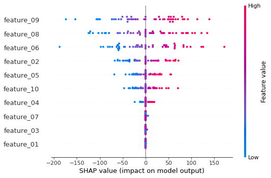
Summary Plot Notes:
Based on the above summary plot we can see that Features 01, 03, and 07 are the features that have no influence on the model and could be dropped (Note that in the data setup we chose 10 features and only 7 of them had a meaningful relationship with the labels/targets). This is the big advantage of SHAP since without this we would not have much insight into which features are actually influencing our model.
The above setup with the dropdown menu allows us to choose the individual labels to explore in more detail.
Force Plot for the first 50 individual examples.
[18]:
print(f"Current Label Shown: {list_of_labels[current_label.value]}\n")

# print the JS visualization code to the notebook
shap.initjs()

shap.force_plot(
    base_value=explainer.expected_value[current_label.value],
    shap_values=shap_values[current_label.value],
    features=X.iloc[0:50, :],
)
Current Label Shown: labels_01
[18]:
Have you run `initjs()` in this notebook? If this notebook was from another user you must also trust this notebook (File -> Trust notebook). If you are viewing this notebook on github the Javascript has been stripped for security. If you are using JupyterLab this error is because a JupyterLab extension has not yet been written.
Reference
Multi-output regression model format/build was largely based on Deep Learning Models for Multi-Output Regression