Fitting a Linear Simulation with XGBoost

This notebook uses SHAP to demonstrate how XGBoost behaves when we fit it to simulated data where the label has a linear relationship to the features.

import numpy as np
import pandas as pd
import xgboost
from sklearn.model_selection import train_test_split

import shap

Build a simulated dataset with linear labels

N = 10000
M = 10
np.random.seed(0)
X_raw = np.random.randn(N, M)
feature_names = [f"feature {i}" for i in range(M)]
X = pd.DataFrame(X_raw, columns=feature_names)
beta = np.random.randn(M)
y = X_raw @ beta

X_train, X_test, y_train, y_test = train_test_split(X, y)
X_strain, X_valid, y_strain, y_valid = train_test_split(X_train, y_train)

Build an XGBoost regressor

Train a depth 1 model

model_depth1 = xgboost.XGBRegressor(
    max_depth=1,
    learning_rate=0.01,
    subsample=0.5,
    n_estimators=10000,
    base_score=y_strain.mean(),
    early_stopping_rounds=20,
)
model_depth1.fit(
    X_strain,
    y_strain,
    eval_set=[(X_valid, y_valid)],
    verbose=1000,
)

[0]     validation_0-rmse:2.17988
[1000]  validation_0-rmse:0.95726
[2000]  validation_0-rmse:0.60452
[3000]  validation_0-rmse:0.41705
[4000]  validation_0-rmse:0.30822
[5000]  validation_0-rmse:0.24119
[6000]  validation_0-rmse:0.19857
[7000]  validation_0-rmse:0.17118
[8000]  validation_0-rmse:0.15386
[9000]  validation_0-rmse:0.14333
[9999]  validation_0-rmse:0.13717

XGBRegressor(base_score=np.float64(0.013271975120564444), booster=None,
             callbacks=None, colsample_bylevel=None, colsample_bynode=None,
             colsample_bytree=None, device=None, early_stopping_rounds=20,
             enable_categorical=False, eval_metric=None, feature_types=None,
             feature_weights=None, gamma=None, grow_policy=None,
             importance_type=None, interaction_constraints=None,
             learning_rate=0.01, max_bin=None, max_cat_threshold=None,
             max_cat_to_onehot=None, max_delta_step=None, max_depth=1,
             max_leaves=None, min_child_weight=None, missing=nan,
             monotone_constraints=None, multi_strategy=None, n_estimators=10000,
             n_jobs=None, num_parallel_tree=None, ...)

In a Jupyter environment, please rerun this cell to show the HTML representation or trust the notebook.
On GitHub, the HTML representation is unable to render, please try loading this page with nbviewer.org.

Train a depth 3 model

model_depth3 = xgboost.XGBRegressor(
    learning_rate=0.02,
    subsample=0.2,
    colsample_bytree=0.5,
    n_estimators=5000,
    base_score=y_strain.mean(),
    early_stopping_rounds=20,
)
model_depth3.fit(
    X_strain,
    y_strain,
    eval_set=[(X_valid, y_valid)],
    verbose=500,
)

[0]     validation_0-rmse:2.17743
[500]   validation_0-rmse:0.27682
[1000]  validation_0-rmse:0.22374
[1500]  validation_0-rmse:0.21615
[1655]  validation_0-rmse:0.21504

XGBRegressor(base_score=np.float64(0.013271975120564444), booster=None,
             callbacks=None, colsample_bylevel=None, colsample_bynode=None,
             colsample_bytree=0.5, device=None, early_stopping_rounds=20,
             enable_categorical=False, eval_metric=None, feature_types=None,
             feature_weights=None, gamma=None, grow_policy=None,
             importance_type=None, interaction_constraints=None,
             learning_rate=0.02, max_bin=None, max_cat_threshold=None,
             max_cat_to_onehot=None, max_delta_step=None, max_depth=None,
             max_leaves=None, min_child_weight=None, missing=nan,
             monotone_constraints=None, multi_strategy=None, n_estimators=5000,
             n_jobs=None, num_parallel_tree=None, ...)

In a Jupyter environment, please rerun this cell to show the HTML representation or trust the notebook.
On GitHub, the HTML representation is unable to render, please try loading this page with nbviewer.org.

Explain the depth 1 model

explainer_depth1 = shap.TreeExplainer(model_depth1)
shap_values_depth1 = explainer_depth1(X_test)

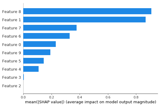
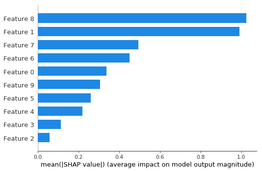
Bar plot shows the global importance of each feature

shap.plots.bar(shap_values_depth1)

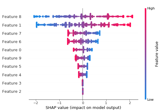
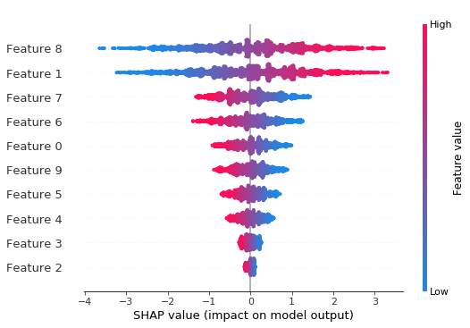
Beeswarm plot shows the global importance of each feature and the distribution of effect sizes

shap.plots.beeswarm(shap_values_depth1)

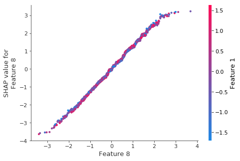
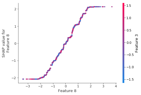
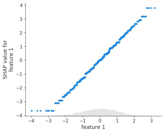
The scatter plot for the top feature shows that XGBoost captured most the linear relationship

It is important to note that XGBoost (and other gradient boosted tree models) is biased towards flat regions, which can be seen below by the flattened tails of the linear function.

# Get the index of the feature with the largest mean absolute SHAP value
top_feature_idx = np.argmax(np.abs(shap_values_depth1.values).mean(0))
shap.plots.scatter(shap_values_depth1[:, top_feature_idx])

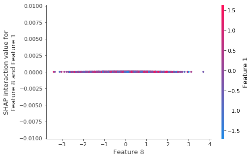
As expected there are no interactions for the depth-1 model:

We can also see this from the lack of any vertical dispersion in the scatter plot above.

# For depth-1 model, interaction values are essentially zero between features
# The second feature index (1) for the interaction plot
second_feature_idx = 1
shap.plots.scatter(shap_values_depth1[:, top_feature_idx], color=shap_values_depth1[:, second_feature_idx])

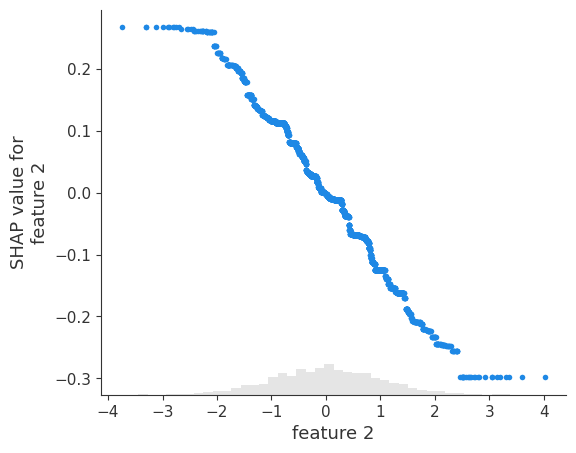
The tail flattening behavior is consistent across all other features.

shap.plots.scatter(shap_values_depth1[:, 1])

Note that weaker signal lead to more variability in the fits:

Since XGBoost likes flat regions the variability will often look like step functions. Remember in the plot below the SHAP values are correctly telling you what the model learned, but the model did not learn a smooth line.

shap.plots.scatter(shap_values_depth1[:, 2])

Explain the depth 3 model

The depth 3 model allows for much richer interactions and should do a better job of fitting the linear function.

explainer_depth3 = shap.TreeExplainer(model_depth3)
shap_values_depth3 = explainer_depth3(X_test)

Bar plot for depth 3 model

shap.plots.bar(shap_values_depth3)

Beeswarm plot for depth 3 model

shap.plots.beeswarm(shap_values_depth3)

The depth 3 model fits the linear function much better

# Get the index of the feature with the largest mean absolute SHAP value for depth 3 model
top_feature_idx_d3 = np.argmax(np.abs(shap_values_depth3.values).mean(0))
shap.plots.scatter(shap_values_depth3[:, top_feature_idx_d3])